1) General principles of the SSE method

1.1) A classical example

As a warm-up before considering the SSE method for solving quantum statistical mechanics problems, we first look at a classical analogue, which will provide a simpler framework for giving insights into some of the key aspects of the method. Consider a classical thermal expectation value

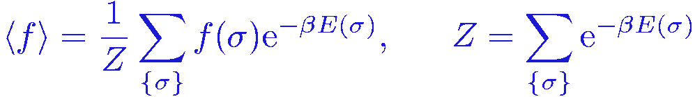
where &sigma includes all the degrees of freedom of the system, e.g., the spin configurations of an Ising model; &sigma={&sigma₁,&sigma₂,...,&sigma_N} , E(&sigma) is the energy, and &beta=1/T is the inverse temperature (using dimensionless units).

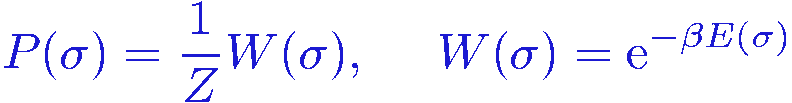
We can evaluate this expectation value using the standard Monte Carlo method, where the configurations are importance sampled, using e.g., the Metropolis algorithm, according to the Boltzmann probability distribution,

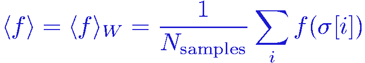
The expectation value is then simply obtained as the average of the function f(&sigma) over the sampled configurations &sigma[i], i=1,...,N_samples

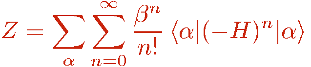
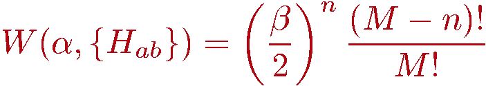
Imagine now that we are not able to evaluate the exponential function. If we are able to evaluate any power of a number, we could Taylor expand the exponential and write the expectation value as

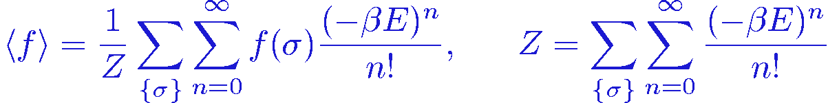
We can think of this as having enlarged our configuration space into an "expansion dimension" where the coordinate to be sampled is the power n. We can thus carry out a Monte Carlo sampling in the configuration space {(&sigma,n)}. This would work provided that all the terms in the sum are positive, which would require the energy to always be negative. This would normally not be the case, but we can always subtract a constant &epsilon from the energy without changing the physics. With a thus suitably chosen constant &epsilon>0, the weight to be used for sampling the extended configuration space is

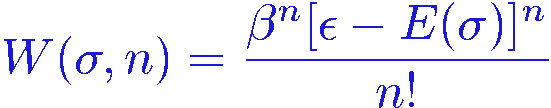
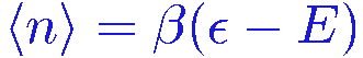
Let's now look at some particular expectation values. The estimator f(&sigma) to be averaged is some function of the original state variables, which does not depend on the expansion power n. However, if f(&sigma) is a function of the energy it turns out that one can rewrite the estimator into a function of only n! To simplify the notation we define H=&epsilon-E.

Let's look at the expectation value <H> of the energy itself:

By shifting the summation index to m=n+1 in the first sum, it is now easy to see that we can rewrite it as

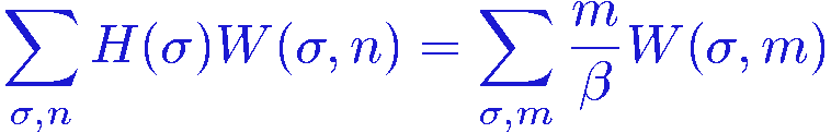
and we can therefore write the expectation value as

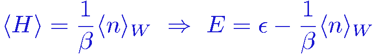
and so indeed we only have to keep track of the expansion power n in order to evaluate the energy. Although a simple result, this is quite remarkable! Of course we still have to deal with the variables &sigma when sampling the configurations.

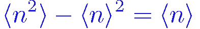
Let's also calculate the expectation value of H². Proceeding as above, writing the sum over n of H²W(&sigma,n) in terms of a shifted summation index k=n+2, we get

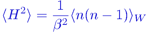
and since the heat capacity C = ( <E²> - <E>² )/T² = (<H²> - <H>² )/T² we have

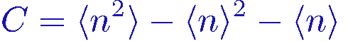
The above expressions for E and C in terms of n are also useful for understanding what expansion powers can be expected to dominate in the sampling. From the expression for the energy E we get the average expansion power

Since &epsilon-E(&sigma) is positive for all states &sigma this expectation value is of course always positive by construction.

Using the expression for C and E together with the above equation we get the variance

Normally C vanishes as the temperature is taken to zero and then we can write the variance as

Since the energy is proportional to the system size N, we can deduce that at low temperarures the average expansion power is proportional to N/T and the width of the distribution is the square-root of the average length. As we shall see, these results will hold true also in the quantum mechanical case.

1.2) Quantum mechanical SSE

In quantum statistical mechanics we are interested in calculating the expectation value of some operator A at temperature T for some model hamiltonian H;

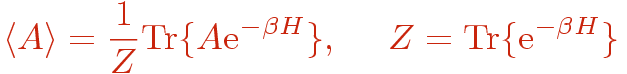
where &beta=1/T and we will work in units where all constants of nature are set to unity. The problem here is how to evaluate the exponential function of the hamiltonian, which in cases of interest contains non-commuting operators. In the SSE method the exponential operator is taken care of by a Taylor expansion and the trace is expressed as a sum over a complete set of states in asuitable chosen basis;

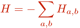
The hamiltonian of interest is written as

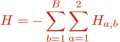
where the indices a and b refer to an operator class or type, e.g., diagonal (a=1) or off-diagonal (a=2) in the chosen basis and a lattice unit, e.g., a bond b connecting a pair of interacting sites i(b),j(b). Tthere can in principle be several types of diagonal and off-diagonal operators; the index a then takes more than two values. The powers of the hamiltonian are written as a sum over all possible products ("strings") of the operators H_ab;

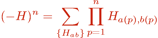
The operators H_ab do not all commute with each other. The order of the operators in the string is therefore important.

It is convenient not to have to deal with strings of varying length n. Therefore, an identity operator 1 that is not part of the hamiltonian is also introduced and written using the same notation as for the terms of the hamiltonian, with indices a=b=0;

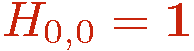
The Taylor expansion is truncated at some cut-off M which is chosen (automatically by the program) sufficiently large for the truncation error to be exponentially small and completely negligble (which can be shown to require M proportional to &beta|E|, where E is the total internal energy). The unit operator H_0,0 is used to augment all strings with n < M. Allowing for all possible placements of unit operators in the string we have

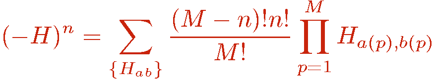
where n now denotes the number of hamiltonian operators in the string, i.e., the operators with non-zero a and b. It should be noted that the truncation of the expansion is not necessary in principle. Simulations can also be done with fluctuating string lengths with no upper bound on n. The importance sampling would then anyway ensure that the range of expansion powers n is finite in practice, because the weight above some power, n>M, is exponentially small and would never be sampled (during the life time of the simulator, or even of the universe). Thus the truncation should not be seen as an approximation. It is introduced as a means for slightly simplifying the sampling scheme. The starting point of the SSE algorithm is thus normally the partition function written as

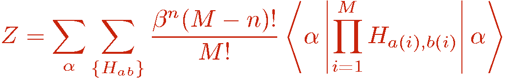
and a similar expression including the operator A in front of the product. In a Monte Carlo simulation, the SSE terms (&alpha,{H_ab}) are sampled according to their weight in the above partition function summation. This requires that all terms are positive, so that they can be used as relative probabilities. The presence of negative terms is referred to as the sign problem. In principle the series can be sampled even with a sign problem, by using the absolute value of the weight and later correcting for the error made, but in practice such simulations are limited to very small lattice sizes. Fortunately there are several classes of interesting hamiltonians for which positive definitness can be achieved.

2) SSE algorithm for the S=1/2 Heisenberg model

The Heisenberg hamiltonian is

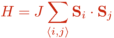
where we assume here that there are interactions only between nearest-neighbor spins, pairs of which are denoted as i,j and we consider the antiferromagnetic case; J>0. The SSE method is by no means restricted to this case, but in order for the expansion to be positive definite (i.e., to avoid the Monte Carlo "sign problem") the lattice has to be bipartite (non-frustrated). A bipartite lattice/interaction is one for which one can divide the sites into two groups, A and B, such that all antiferromagnetic interactions are between sites in A and B. This is the case for the 2D square lattice (or a cubic lattice in any D) with nearest-neigbor interactions, for which the sublattices corresponds to the black and white squares of a checkerboard, as illustrated in the figure below with red and blue sites. A prototypical example of a non-bipartite (frustrated) lattice is the triangular lattice.

The program ssebasic.f90 is written for the 2D square lattice with N=Lx*Ly sites and periodic boundary conditions. Note that Lx and Ly both have to be even for this lattice to be bipartite.

We will use the standard basis of spins "up" and "down" along the z quantization axis. For a lattice with N spins (S=1/2) the basis states are thus

In this basis it is convenient to rewrite the hamiltonian using the z-component and ladder operators, and we also set the coupling J=1)

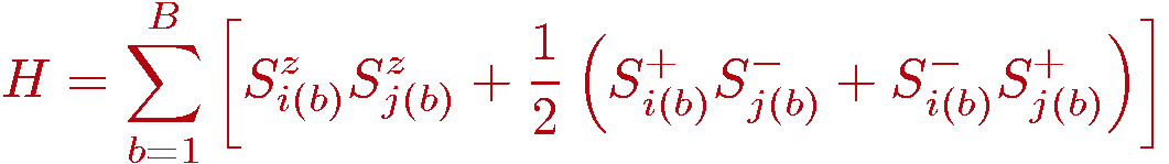
where we have also introduced the bond operator notation; b=1,...,B denotes a bond connecting two interacting spins i(b),j(b) and B is the number of bonds. For the 2D square lattice with periodic boundary conditions B=2N.

We now introduce the diagonal (a=1) and off-diagonal (a=2) bond operators

in terms of which the hamiltonian is

Here we have neglected a minus sign in front of the off-diagonal operators. This corresponds to a sublattice rotation, in which all the ladder operators are multiplied by -1 (or, equivalently, the x and y spin operators are rotated by 180 degrees) on one of the sublattices of a bipartite lattice. The sublattice transformation does not affect the commutation relations among the spin operators and hence the level spectrum of the hamiltonian does not change. Physical properties involving off-diagonal operators change only, at most, by a sign. The ability to carry out such a transformation is what enables a positive-definite expansion in the SSE method. For a non-bipartite lattice there will be both positive and negative terms in the expansion and the Monte Carlo sampling is then hampered by the sign problem. We will se below that the positive definitness for a bipartite lattice also follows automatically in the SSE method even without formally carrying out a sublattice rotation, i.e., we could equally well keep the minus sign of the off-diagonal operators and still obtain a positive definite expansion. We will anyway leave out the sign here to make the formulas a bit simpler. Thus the assumption here is always that we are dealing with a bipartite lattice. The reason for introducing the constant 1/4 in the diagonal bond operator also has to do with avoiding a sign problem, as will become clear below.

2.1) Representation of operators and states; SSE configurations

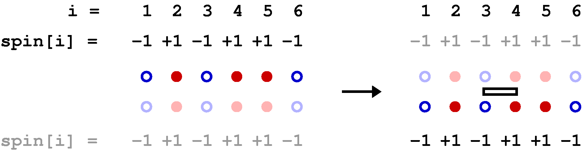
In the program the SSE operator products in the partition function,

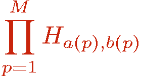
are represented by a one-dimensional integer array opstring[p], p=1,...,M, where both indices a and b are encoded into a single integer according to:

so that even and odd valued elements correspond to diagonal and off-diagonal operators, respectively. The non-hamiltonian identity operator (a=b=0) is naturally encoded as: opstring[p]=0.

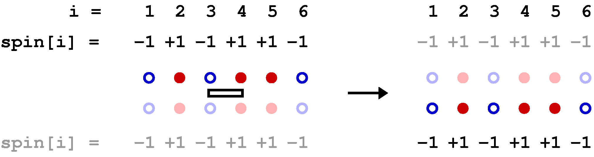
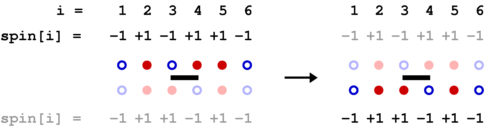
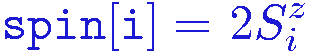
The spin state |&alpha> of the system is represented by an array spin[i], i=1,...,N, with elements +1 and -1 corresponding to spin up and down, or

The bond index b corresponds to two interacting spins i(b),j(b), which in the program are stored in an array bsites(s,b), where s=1,2 corresponds to the two sites; bond b connects sites bsites[1,b] and bsites[2,b]. This list is the only information on the lattice geometry needed in the sampling of configurations. For the bond labeling, the program ssebasic.f90 defines the x-bonds in the range b=1,...,N and the y-bonds in b=N+1,...,2N. The sites with coordinates x=0,...,Lx, y=0,...,Ly on an Lx*Ly lattice are numbered as i=1+x+y*Lx, but this information does not have to be stored as it is not needed in the simulation. The coordinates can be needed in various measurements, but then they can easily be calculated on the basis of the site index i; x=mod(i-1,Lx), y=(i-1)/Lx. The labeling convention for sites and bonds for a 4*4 lattice are shown in the figure below.

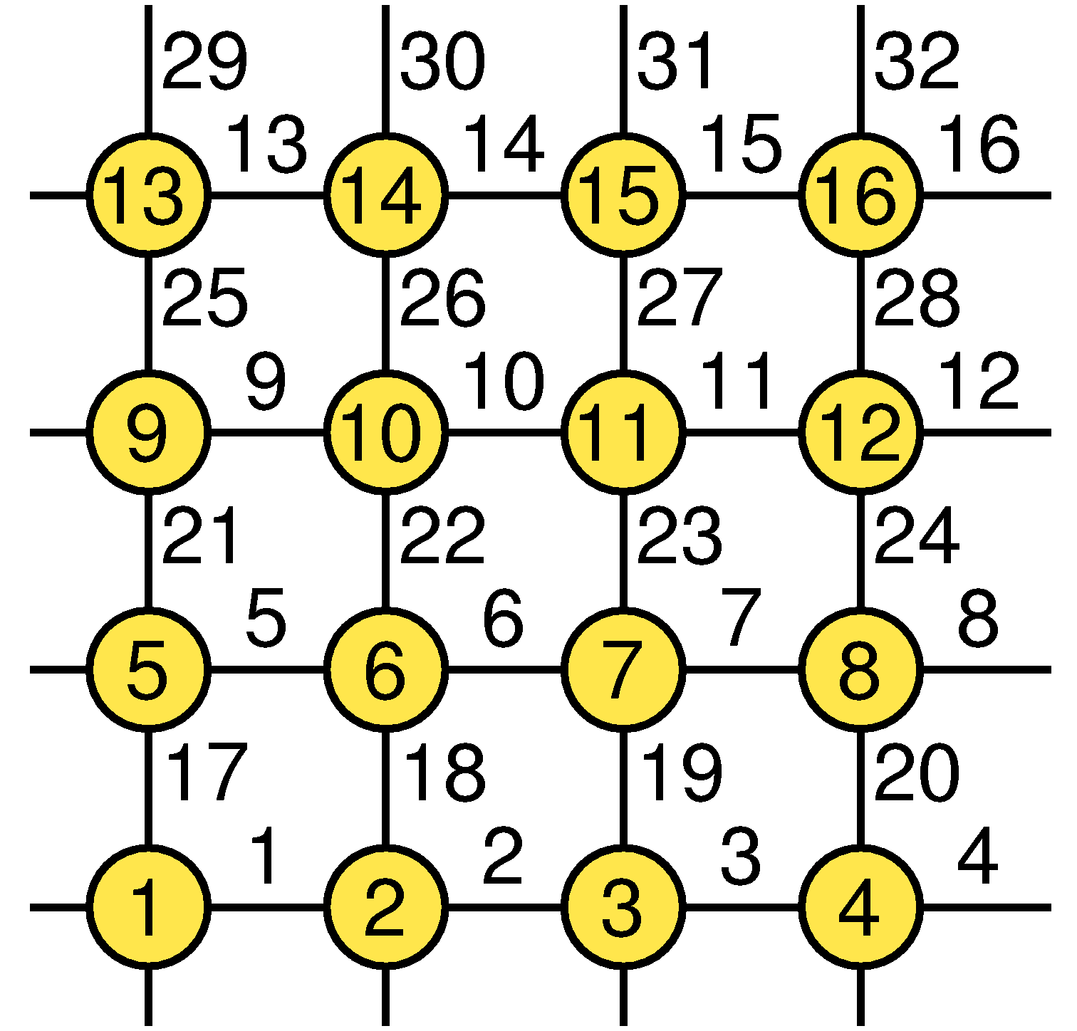
Thus bsites[1,1]=1,bsites[2,1]=2,...,bsites[1,4]=4,bsites[2,4]=1,..., bsites[1,17]=1,bsites[2,17]=5,...,bsites[1,32]=16,bsites[2,32]=4.

With the constant 1/4 included in the definition of the diagonal operator, both types of operators (diagonal and off-diagonal) can act only on anti-parallel spins, i.e., any operator acting on a pair of parallel spins leads to a configuration that does not contribute to the partition function. This is a key aspect of the SSE method for the isotropic S=1/2 Heisenberg model. Another key aspect is that all non-zero matrix elements of both diagonal and off-diagonal operators equal 1/2, so that the weight W of an allowed configuration (&alpha,{H_a,b}) is simply given by the number, n, of non-unit operators in the sequence;

In the simulation the configurations are to be sampled with a probability proportional to this weight; P=W/Z. It is thus clear that a constant had to be added to the bond operator and that its minimum value is 1/4, in order to make W positive definite. The value 1/4 for the constant is particularly practical (exactly why will become clear later) because it disallows operation on parallel spins, which is also the case with the spin-flipping off-diagonal operators.

It is useful to define a propagated state |&alpha(p)> as the stored basis state |&alpha>=|&alpha(0)> propagated by the first p operators in the string;

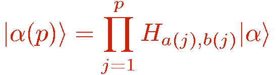
These states are of course also basis states. This is another key aspect of the SSE method; that the operators and basis have to be chosen such that propagating a basis state with an operator string leads to a sequence of single basis states, i.e., there is no branching of "paths".

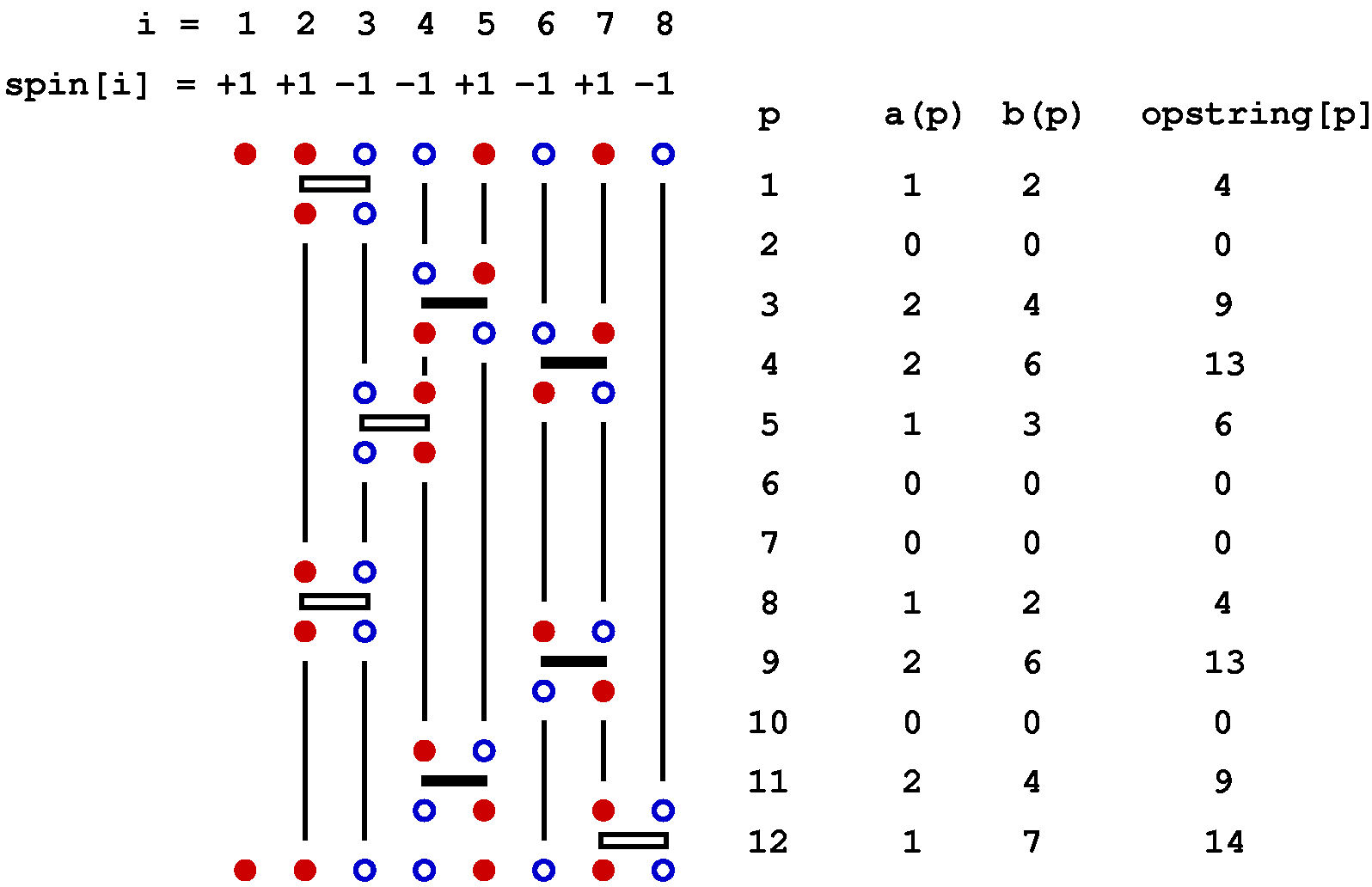
Below is a graphical representation of an SSE configuration for a 8-site one-dimensional chain, showing all the propagated states. Each row of red and blue circles corresponds to a state of spins up (red) and down (blue). The operators are represented by bars between the sites on which they act; open and solid bars for diagonal and off-diagonal operators, respecyively. In this case the expansion cut-off M=12, there are n=8 hamiltonian bond operators and, four (M-n=4) unit operators (a=b=0). The latter correspond to empty space between the states where these operators "act". The figure also shows the data structures stored in the computer, along with the indices a(p) and b(p), which are not stored but are easily obtained from the operator string when needed; a(p)=MOD(opstring[p],2)+1, b(p)=opstring[p]/2. The bond index b in this one-dimensional example equals the site label of the first spin connected by the bond, i.e., bond b is connected to sites b and b+1.

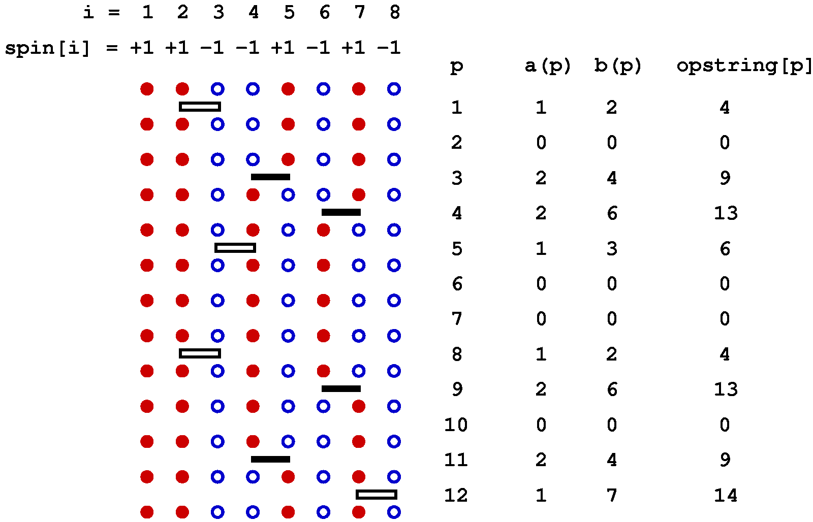
The propagated states are not stored in the program but are shown explicitly here in order to illustrate how the operator string propagates the state |&alpha> periodically, i.e., the boundary condition |&alpha(M)> = |&alpha(0)> = |&alpha> must be satisfied for a contributing configuration. This periodicity implies that each spin must be flipped an even number of times (or not at all) during the propagation from p=1 to p=N. This in turn implies that there has to be an even number of off-diagonal operators in the string. Thus, even if we had kept the minus sign in front of the off-diagonal operators, this sign would never show up because it would be raised to an even power in all allowed configurations. For a non-bipartite lattice this is no longer true, as sn odd number of oparators then can flip spins cyclically around a loop, in such a way that each spin is flipped twice and hence leaving the spins on the loop the same as before the propagation.

Clearly the vast majority of configurations do not satisfy the periodicity and hence do not contribute to the partition function. A requirement for an efficient sampling scheme for the configurations is that no attempts to change the configuration are carried out that violate the propagation periodicity.

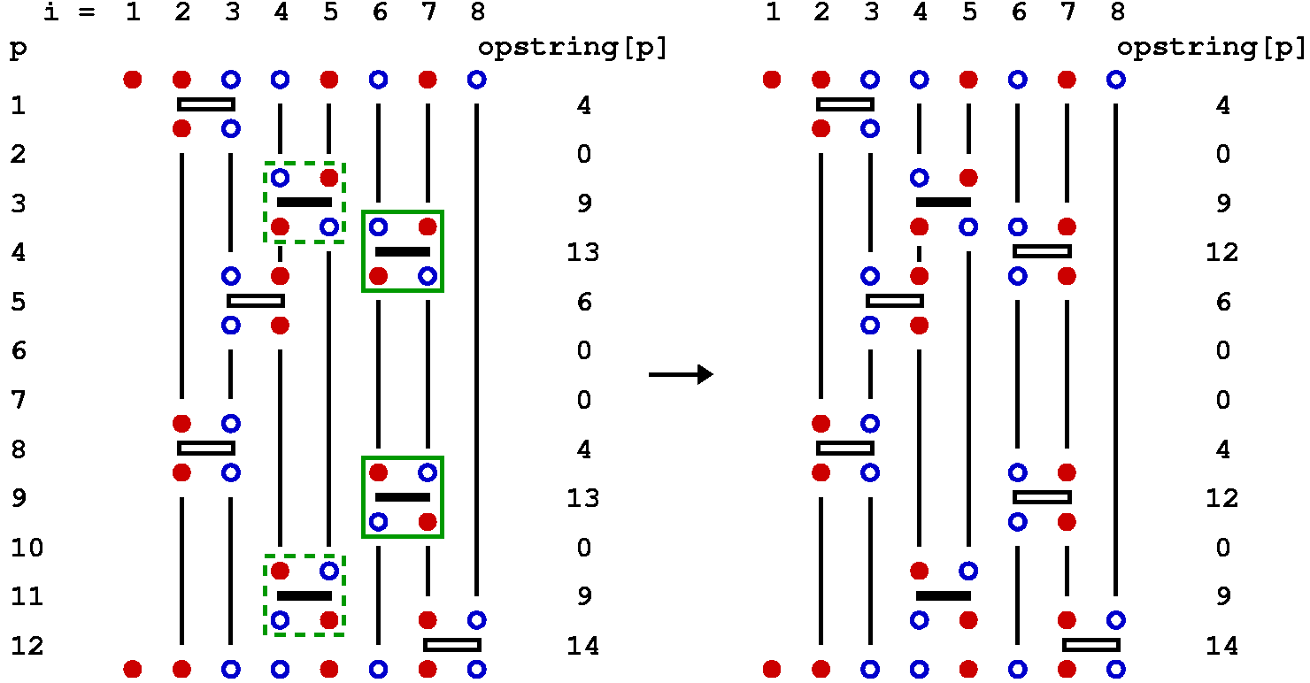
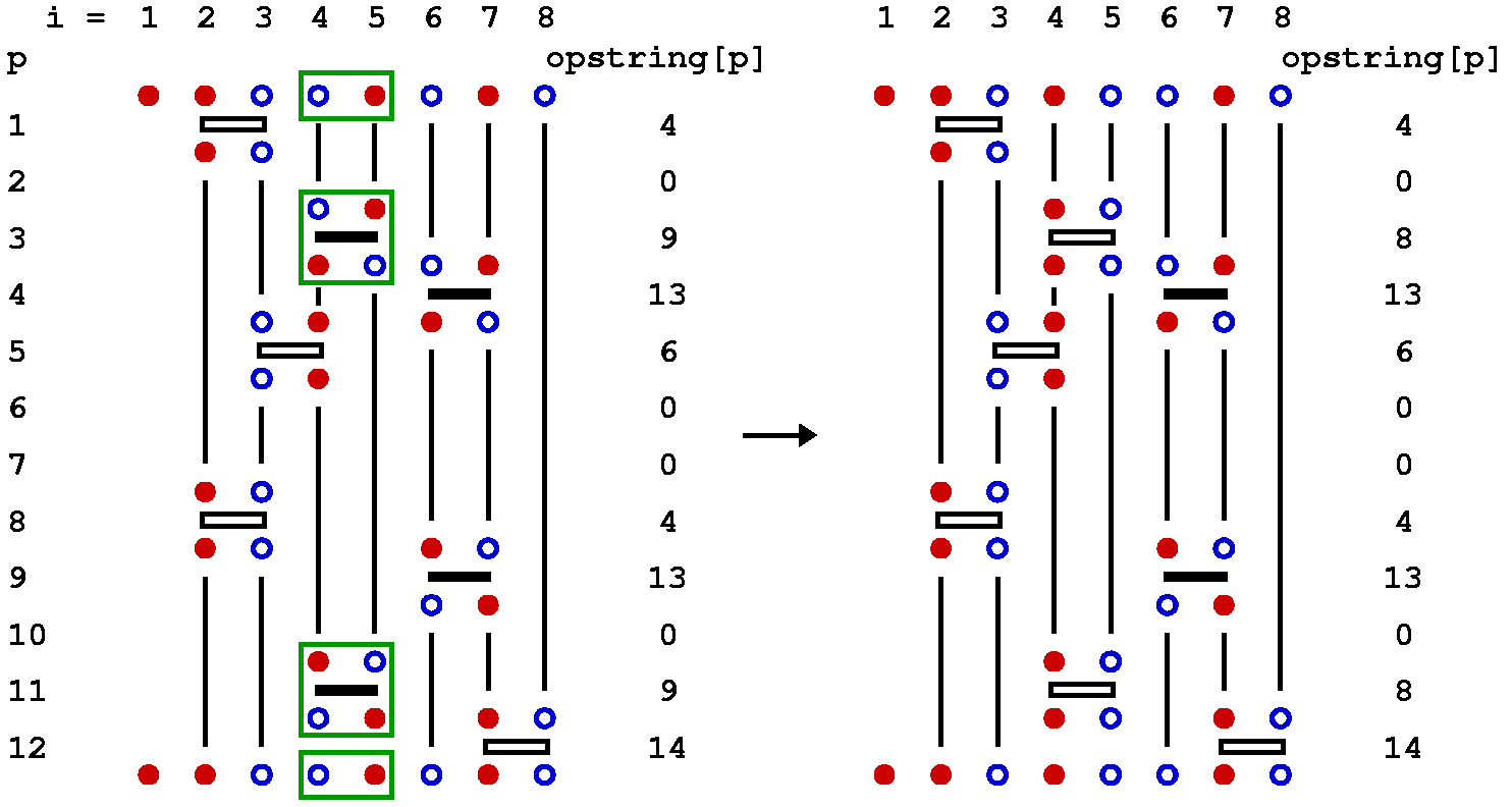
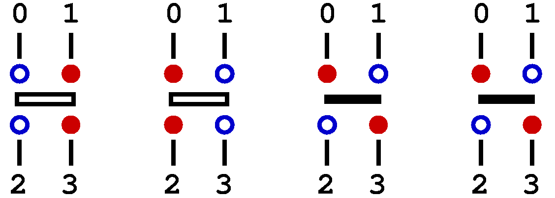
The representation of the current SSE configuration by the arrays spin[] and opstring[] is used throughout the program. From these, any propagated state can be generated as needed. In one part of the updating procedure another temporary representation of the configuration is used. This linked vertex representation captures directly the way the operators are "connected", i.e., using it one can directly jump from an operator at position p, which acts on two spins i(b(p)) and j(b(p)) (in the program bsites[1,opstring[p]/2] and bsites[2,opstring[p]/2) to the next or previous operator acting on one of these spins, without having to conduct a tedious search in the list opstring[]. Each bond operator acts on two "in" spins and the result of this operation is two "out" spins. In the linked vertex representation an an operator is represented by a vertex with four legs. Each leg has a corresponding spin state. There are four allowed vertices;

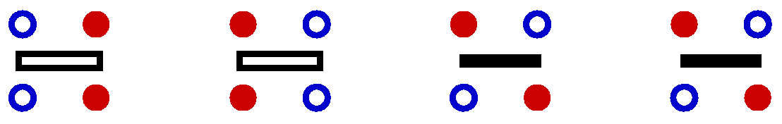
Here the bars between the spins are clearly redundant, but for illustrative purposes it is useful to keep them anyway.

A graphical representation of the linked vertices is obtained by removing from the propagated states in the full-configuration figure above the columns of fixed spins between consecutive operations. These spins are replaced by vertical lines, representing links between elements in a list kept in the program;

In the linked list one can move from any vertex leg to the next or previous leg sitting on the same site or the other site on which the operator acts. Each vertex can be identified by its position p in the list opstring[]. Labeling the vertex legs l(p)=0,1,2,3 as shown below, any vertex leg can be identified by an integer v=4*(p-1)+l(p).

The linked list is a temporary data structure, to be used in one of the configuration updates. It is constructed before this update and destroyed after. The data structutes opstring[] and spin[] serve as permanent storage of the configuration. In the program, the link connecting vertex leg v is stored in a list vertexlist[v], v=1,...,4*M. Here we describe the contents of the list, deferring to the following section the discussion of how and why it is used. The procedures for constructing the linked list using the information in opstring[] and spin[] will be discussed in the program description, Sec. 4.

The list element vertexlist[v] contains the label (i.e., the position in vertexlist[]) of the vertex leg to which leg l=MOD(v,4) of vertex p=1+(v-1)/4 is connected. The list is double-linked, so that one can move both up and down. This implies that vertexlist[vertexlist[v]]=v. For the configuration illsutrated above, the contents of the vertex list are,

                  l =  0         1         2         3           p
                                                            
[v] vertexlist[v]:   [ 1] 31   [ 2] 32   [ 3] 29   [ 4] 17       1
                     [ 5]  0   [ 6]  0   [ 7]  0   [ 8]  0       2
                     [ 9] 43   [10] 44   [11] 18   [12] 42       3
                     [13] 35   [14] 47   [15] 33   [16] 34       4
                     [17]  4   [18] 11   [19] 30   [20] 41       5
                     [21]  0   [22]  0   [23]  0   [24]  0       6
                     [25]  0   [26]  0   [27]  0   [28]  0       7
                     [29]  3   [30] 18   [31]  1   [32]  2       8
                     [33] 15   [34] 16   [35] 13   [36] 45       9
                     [37]  0   [38]  0   [39]  0   [40]  0      10
                     [41] 20   [42] 12   [43]  9   [44] 10      11
                     [45] 36   [46] 48   [47] 14   [48] 46      12

2.2) Sampling the configurations; diagonal, loop, and single-spin updates

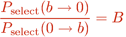
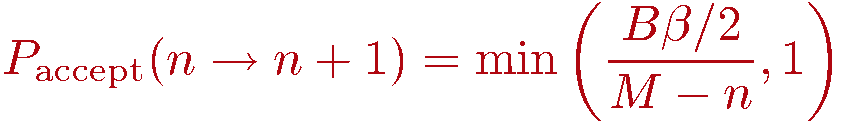
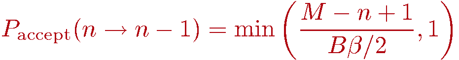
We now discuss how to generate configurations in the representation outlined above. As always in Monte Carlo importance sampling, we start from some arbitrary allowed configuration (i.e., with nonzero weight W) and from it generate a Markov chain of configurations by making changes (updates of the configuration) that are accepted or rejected according to probabilities chosen so that detailed balance is satisfied and thus the desired probability distribution P=W/Z is sampled. Using the Metropolis method, the probabilities to accept a tentative change of the old configuration into the tentative new one is

The decision of whether to accept the update if P_accept < 1 is of course made by comparing with a random number R in the range [0,1); If R>P_accept the update is rejected and the old configuration is kept.

One also has to pay attention to how the tentative changes are done: With the above Metropolis acceptance probability, the probability of making a tentative change from a current configuration A to a new configuration B must be the same as the probability of making the tentative change to A when the current configuration is B. If this is not the case, then the acceptance probability has to be modified in order to correct for the imbalance. In simple classical Monte Carlo simulations, e.g., of the Ising model, the tentative probabilities are trivially equal, e.g., when randomly selecting a spin i to flip (i.e., tentatively flipping it) the selection probability is always the same; P_select(i)=1/N. As we shall see below, this is not always the case when updating an SSE configuration.

Consider two configurations A and B, for which there is an update that can change them into each other. If the probability for selecting B when in A is not the same as selecting A when in B, one can use the acceptance probability

In the SSE method for the Heisenberg model, three types of updates are used, called diagonal update, single-spin flip, and loop update. The diagonal update is carried out using the representation in terms of the operator string opstring and spin[], whereas the loop update and the single-spin update make use of the linked vertex list vertexlist[], which hence is constructed before this update is carried out. We will also discuss an off-diagonal pair update update, which is typically not used because the loop update is much more efficient. We will discuss it here because it helps in understand the fine points about the loop update.

The simulation can be started from an arbitrary allowed configuration, e.g., an "empty" string (containing only elements 0, and thus n=0) of arbitrary length M and a random spin state. The cut-off M will later have to be adjusted. This will be discussed after we have described the different types of updates.

Diagonal update

The purpose of the diagonal update is to change the number n of hamiltonian operators in the sequence. The simplest way to do this is to substitute unit operators opstring[p]=0 by diagonal operators opstring[p]=2*b and vice versa. While one can always substitute a diagonal operator by a unit operator and obtain a new valid configuration, the insertion of a diagonal operator acting on a bond b requires that the spins at this bond are in an antiparallel state in the propagated state |&alpha(p)>. Hence one has to keep track of the propagated states. It is then natural to carry out the diagonal updates sequentially, starting at p=1 and propagating the state stored in spin[] as off-diagonal operators are encountered. Off-diagonal operators cannot be inserted or removed one-by one and they are thus left unchanged in this update.

We look at the three possible actions to be taken at step p of the diagonal update: At the start of the cycle of diagonal updates the spins stored in spin[] are those of the state |&alpha> = |&alpha(0)>.

We also have to consider the probability of selecting the bond b, which is 1/B. This is different from the selection of the opposite move where we select the unit operator with probability one when removing a diagonal operator. The ratio is

and thus the acceptance probability is

If the outcome of the random decision is the accept, then we update the operator element; opstring[p]=2*b and increment n; n=n+1. For the next updating step we need the p+1:th propagated state, which in this case is the same as the previous one because the inserted operator is diagonal. Hence we can directly move on to position p+1, regardless of whether the update was accepted or not. This figure illustrates a diagonal update where an operator is successfully inserted. The propagated states before and after operator position p are shown, with the currently stored spin state indicated by the brighter colors and darker text.

Removal of a diagonal operator: This is attempted if we encounter a diagonal operator, i.e., if the stored operator list element is nonzero and even; if MOD(opstring[p],2)=0. This case is very similar to the insertion case, but we do not have to generate any bond index. The weight ratio when n is decreased by one is

and so the acceptance probability is

Again there is no change in the spin state. This is the pictorial representation of the diagonal update of operator removal.

State propagation with an off-diagonal operator: When the encountered operator is an off-diagonal one, i.e., if MOD(opstring[p],2)=1, we cannot carry out a doagonal update. In this case the operator changes the spin state and so we propagate the stored state, using the bond index of the operator at p; =b=opstring[p]/2, which acts on spins s1=bsites[1,b] and s2=bsites[2,b]. These spins are flipped; spin[s1]=-spin[s1], spin[s2]=-spin[s2]. This is the pictorial representation of such a step.

When we have completed the diagonal update at the last position p=M in the string, the stored spins have been propagated back to the original state (because of the periodicity |&alpha(M)>=|&alpha(0)>) and we move on to the next type of update.

Spin flip update

In the full configuration illustrated in several of the figures above, it can be seen that there are no operators acting on site i=1. The spin state at this site is therefore arbitrary and it can be flipped with a fixed probability P, e.g., P=1 or P=1/2 (in some pathological cases P=1 leads to loss of ergodicity). However, at low temperatures it is unlikely to find such "free" spins and therefore no updates of this type will be carried out in practice. In principle, one can also simultaneoulsy flip clusters of spins that are connected by operators, since this maintains the requirement that all operators act on antiparallel spins and no changes in the weight result. But at low temperatures all the spins will most likely belong to the same cluster and then this kind of update is pointless. As we will see below, the state |&alpha> will be changed also without carrying out these spin flip updates so (in most) cases they are strictly not needed .

Off-diagonal pair update

The diagonal update does not, as the name indicates, lead to any changes involving off-diagonal operators, i.e., the propagation path (the sequence of spin states |&alpha(0)>...|&alpha(M)>) does not change. Off-diagonal operators cannot be introduced or removed one at a time, because of the periodicity requirement |&alpha(0)>=|&alpha(M)>), which implies that every spin has to be flipped zero or an even number of times. Off-diagonal operators can be inserted and removed in pairs, by exchanging them with diagonal operators acting on the same bond, as shown in the figure below. This kind of update will be discussed here mainly for pedagocical reasons, as it is, in most cases, not very efficient compared to the loop update which can lead to simultaneous changes in many operators. It is, however, useful to go through it anyway as it illustrates some concepts that are needed later.

The pair of operators enclosed by solid green squares in the configuration to the left can be replaced by diagonal operators, as shown in the configuration to the right, without affecting the periodicity of the path. Furthermore, since the diagonal and off diagonal operators have the same value 1/2 of their non-vanishing matrix elements, such an update can always be accepted according to the Metropolis rule, provided of course that the probability to select the pair is the same in going from the right to left configuration and vise versa (which can be very easily arranged the case). Notice that the columns of spins between the two replaced operators have been flipped in the process.

A pair replacement cannot be done with the operators enclosed by dashed green squares in the left configuration, because there is another operator between the two, at position p=5, which acts on one of the spins, i=3, that will be flipped after the replacement. The diagonal operator would then act on two parallel spins, which is not allowed.

In the statements above, we have to be careful with what exactly we mean by "between" operators. If we imagine propagating the spin state starting from p=1 and increasing p (going down in the figure), then indeed spins 4 and 5 in the propagated states |&alpha(3)> to |&alpha(10)> would be flipped after we change the type of the operators at p=3 and p=11. We would then have created an illegal operation at p=5. However, we can also imagine that we first propagate the stored state |&alpha> to |&alpha(10)> and make the operator changes only after that. After having changed the two operators, we can continue propagating the state, going across the periodic boundaries and continuing to p=2, i.e., generating |&alpha(11)>, |&alpha(12)>=|&alpha(0)>, |&alpha(1)>, |&alpha(2)>. The spins at sites 4 and 5 are then flipped in all these states (relative to the spins before the operator replacement). In this case we do not encounter any other operator acting on sites 4 and 5 until we reach the replaced operator at p=3, and so the pair update is now completely legal. The difference between this way of doing the update and the one illustrated above, which involve exactly the same two operators, is that we in the later case have also changed the stored spin state |&alpha>. If we carry out this replacement of operators we hence also have to flip spin[4] and spin[5]. This update is illustrated in the figure below.

To carry out the pair update, one would thus search for pairs of bond operators acting on the same bond b that do not have any other operators acting on b in between them. The search in the configuration should be done with the periodic boundary conditions |&alpha(M)>=|&alpha(0)> taken into account. This can be conveniently done using the linked vertex list representation of the configuration. Note that the two operators do not necessarily both have to be of the same type. If they are of different type, one diagonal and one off-diagonal, the effect of the update is only to move operators, not to change the numbers n₁ and n₂ of, respectively, diagonal and off-diagonal operators.

To change the operator types diagonal/off-diagonsl in the pair update, the FORTRAN exclusive-or bit operation IEOR(a,1) can be used. This operation has the effect of adding 1 to an even number a and subtracting 1 from an odd a; exactly what we need to change the operator element opstring[p] between diagonal and off-diagonal operators with the bond index unchanged; opstring[p]=IEOR(opstring[p],1).

In practice the pair update is not very efficient; it only makes very small changes in the propagation path whereas the subspace of configurations contributing significantly to the partition function often involve hugely different paths (not only close to critical points). In fact, for a system with periodic boundary conditions this update, in combination with the diagonal update

Operator-loop update

The loop update accomplishes changes in the types of operators diagonal/off-diagonal for a varying number of operators without changes in the bonds on which they operate. In the simplest case, it corresponds exactly to the off-diagonal pair update. The idea is to construct a loop connecting vertex legs as shown in the figure below. Each vertex leg is linked to some other leg and these two form a segment of a path. By extending the path to the legs of these same vertices on the same horizontal level (above or below the operator bar in the figure), and then to the legs they are linked to, etc., a closed loop will eventually be formed. As seen in the configuration to the right, the spins at all the vertex legs covered by this path can be flipped, which, for operators encountered only once, corresponds to changing the operator type, diagonal to off-diagonal and vice versa. For operators encountered twice (which is the case with the one at p=5 in the figure), all four spins are flipped and the operator type then remains unchanged. Clearly, a loop update can affect a very large number of operators and hence it can be expected to be more efficient than the pair update. In addition, the loop update has several other important aspects which will be discussed further below.

It is clear from the picture that each vertex leg uniquely belongs to a single loop. It is thus approporiate to construct all the loops and flip each of them with probability 1/2. This is analogous to the Swendsen-Wang cluster update for the classical Ising model. In the classical case, it is often more efficient to use the Wolff algorithm, where clusters are constructed at random (with different randomly chosen starting sites from which the cluster is built up) and flip them with probability 1. In the case of the SSE operator-loop update, this is not recommended because the loop structure is only changed in the diagonal update. Thus, without carrying out a diagonal update between loop updates one would some times flip the same loop back and forth. The recommended approach is to carry out a cycle of diagonal update followed by the construction of all loops, which are flipped with probability 1/2.

In the linked list representation, the procedure of constructing a loop (regardless of whether it will be flipped or not) is the following: Pick an element v0 in the linked list. This corresponds to position (vertex number) p0=(v0-1)/4+1 in the operator string and vertex leg l0=MOD(v0-1,4). These labels are not needed, however. Now set v1=v0. From v1, we go to the leg to which it is linked, i.e., v2=vertexlist[v1]. We now want to go to the leg on the same vertex as v2 which is on the same level as v2; its neighbor leg. This can simply be obtained as v1=IEOR(v2,1). We then choose v2 to which this v1 is linked, etc. At some point we will reach the original starting point; v2=v0 and the loop then closes. When the loop is constructed we also need to somehow mark the visited legs, and also information on whether or not the loop should be flipped. The random 50/50 decision of whether or not to flip is made before the loop is constructed. The actual loop flip will be made after the loop has been constructed, and only some intermediate information needed at that point will be recorded during the loop construction. Since a given loop should be constructed only once, each leg should be visited exactly once. Thus, after an element v in opstring[] has been visited and we have moved to its neighbor, we are guaranteed not to need the link opstring[]. Thus we can set this element to a number, e.g., 0, if the element has been visited and the loop is not to be flipped and -1 if it should subsequently be flipped.

2.3) Ajusting the expansion cut-off M

3) Measuring operator expectation values

4) Computer program implementation; ssebasic.f90