National High Magnetic Field Lab, Tallahassee, Florida
Theory Winter school, January 9-13, 2012
Anders W. Sandvik, Boston University
Lecture slides Lecture 1 Lecture 2
Detailed review of numerical methods for quantum spin systems (including SSE)
Computational Studies of Quantum Spin Systems, A. W. Sandvik, AIP Conf. Proc. 1297, 135 (2010)
Material for afternoon tutorial, January 11
A basic variant of the Stochastic Series Exapsnion (SSE) Quantum Monte Carlo program is provided here. It computes some essential properties if the S=1/2 Heisenberg model in one and two dimensions.
The lattice size N=Lx*Ly, with the lengths Lx and Ly given by the user as input. In cases where Lx and Ly are not the same, Lx should be the longer size. For Ly=1, the system is then a one-dimensional chain, with periodic boundaries in the x direction. For Ly=2 it is a 2-leg ladder, with periodic boundary conditions in the x direction but not in the y direction (since in this case that would double the effective interaction strength in the y direction). For all other cases the boundaries are periodic in both directions. The figure below summarizes the lattices and boundary conditions.
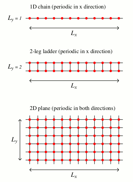
Note that in all cases except the single chain, Lx and Ly should be even numbers (Lx should be even also for the Ly=1 chain). Otherwise there is a sign problem in the simulations, which is not taken into account in this program.
Source codes (Fortran 90) ssebasic.f90 (simulation program; output should be processed by 'res.f90') res.f90 (program to compute averages and error bars from output of ssebasic.f90)
Running instructions
Compile the programs (e.g., with g95 or gfortran).
Input parameter for ssebasic are read from a file 'read.in', in the following format:
    lx, ly, beta
    nbins, msteps, isteps

    lx,ly  : lattice size in x and y direction
    beta   : inverse dimensionless temperature J/T
    nbins  : Number of bins (averages written to file 'res.dat' after each bin
    msteps : Number of MC sweeps in each bin (measurements after each sweep)
    isteps : Number of MC sweeps for equilibration (no measurements)
In addition, a random number seed (integer) is read from 'seed.in'
Output is written after each completed bin to 'res.dat'. Thiese raw data should be processed
by the program 'res.f90'. It produces two files:
- e.dat: internal energy and specific heat (with error bars)
- m.dat: squared sublattice magnetization and uniform susceptibility (with error bars)
In addition, the simulation program also produces a file 'cut.dat' in which the new truncation
of the series expansion is written each time it is increased.
An example
Running the program with these oarameters in 'read.in'
    8   8      2.
    10  10000  10000
Produced the following output (results of 10 bins) in 'res.dat' (after running a few seconds on a MacBook Air):
    -0.60545312499999993       0.45663118750002241       0.12939503187647464       7.49062499999999937E-002
    -0.60682343749999990       0.44244269437507455       0.12865359015698782       7.48968750000000016E-002
    -0.60736640624999993       0.42738905609377298       0.12857748019236501       7.65843749999999962E-002
    -0.60639140624999999       0.47596175609373859       0.13036687638192762       7.63156249999999980E-002
    -0.60511015625000009       0.39663114359370866       0.12531685491597871       7.72062500000000040E-002
    -0.60642031250000006       0.42985882437494638       0.13028933087043010       7.74468749999999984E-002
    -0.60657500000000009       0.52802733499993337       0.13139164458652658       7.64906250000000065E-002
    -0.60733203124999990       0.42871590234381074       0.12873853782797756       7.75593749999999998E-002
    -0.60921562500000004       0.53947162249994562       0.13185469109301354       7.49156249999999996E-002
    -0.60873593750000010       0.53154232437492510       0.12912797510686908       7.72593750000000051E-002
Running 'res.f90' gave this output in e.dat (energy and specific heat)
-0.60694234 0.00040847 0.46566718 0.01608355
and in 'm.dat' (sublattice magnetization squared and susceptibility):
0.12937120 0.00057857 0.07635813 0.00034245
Note that the specific heat is much noisier (has much larger error bar) than the energy. It is
very difficult (requires very long runs to get small error bars) to compute the specific heat at
low temperatures (roughly beta>4)
Test of the correctness of the program
It is important to test QMC programs against exact results, whenever possible. It is always possible to check against exact diagonalization for small systems. As an example, for a chain of L=32 the ground state energy per spin is -0.4439539825. Let's see if we can get agreement with this number by choosing beta=1/T large enough (T should be much smaller than the finite-size gap, which scales approximately as 1/L). These are results versus beta using 20 bins of 100000 MC steps each:
    1.0    -0.20477922     0.00016893
    2.0    -0.34135748     0.00016988
    4.0    -0.41897368     0.00007303
    8.0    -0.43776850     0.00003716
   16.0    -0.44240240     0.00002830
   32.0    -0.44377160     0.00002360
   64.0    -0.44394747     0.00002178

   exact   -0.44395398
The last two data points agree with the exact results within error bars (here in the fifth digit).
Note that beta was successively doubled, which is useful when one wants to check the
convergence in calculations aimed at the ground state. Note also that the error bar decreases
with increasing beta. This is because the 'imaginary time' dimension of the system increases,
and the energy (estimated using the average length of the expansion) is automatically averaged
over the whole space-time volume. For the largest beta this calculation took about 5 minutes
on a MacBook Air.
Specific task for the tutorial
As seen above, if beta is chosen sufficiently large, for a given system size, one obtains ground state results. The squared sublattice magnetization m2 contains information on the spin correlations in the system. By studying it as a function of the system size one can see the nature of the ground state.
Do simulations of chains (size L*1) 2-leg ladders (size L*2) and 2D systems (L*L) at inverse temperature beta=2*L. This will be sufficient to obtain ground state results affected only very little by remaining finite-temperature effects. Do 10 bins with 10000 MC sweeps in each bin and 10000 sweeps for equilibration. Within reasonable simulation time (up to minutes) you can then go to something like L=32 to L=64 for the chains and ladders, and maybe up to L=16 for the 2D systems. Do several L for each case (and remember that L has to be even!).
For the chains and ladders, plot L*m2 versus L and for the 2D systems plot m2 versus L. The behaviors can be explained by the form of the spin-spin correlation function C(r) as a function of the distance r in these systems: In the chain C(r) decays as 1/r (with a log correction that slightly affects the results), in the ladder the decay is exponential with r, and in 2D C(r) approaches a non-zero constant for large r (the square of the sublattice magnetization of the infinite system). The computed sublattice magnetization is the sum of C(r) over all r on the lattice, divided by N.
Results obtained by Ying Tang:
Some of this material is based upon work supported by the National Science Foundation under Grant Nos. DMR-0803510 and DMR-1104708. Any opinions, findings, and conclusions or recommendations expressed in this material are those of the author(s) and do not necessarily reflect the views of the National Science Foundation