Solution program (Fortran) [eq.f90]

Part 1 (averaged magnetization)

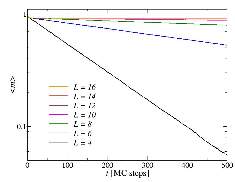
at T = 2 < Tc, graphing the average magnetization as a function of the simulation time on a lin-log scale we can see that asymptotically the decay is exponential. The time-constant of the decay becomes very large (diverges) as L increases, so that an equilibrium value of the magnetization is established on practical time scales when the system is large. Here the equilibrium value is about =0.91.

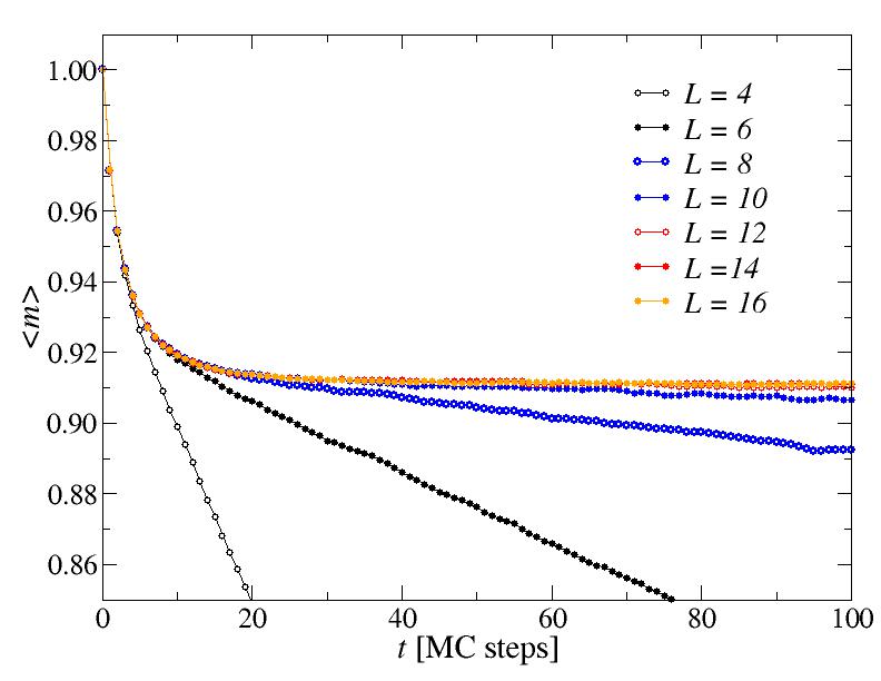
There is a different time scale associated with the approach to the equilibrium value, which we can see if we focus in on the short-time behavior. At this temperature that time scale is just a few Monte Caro steps.

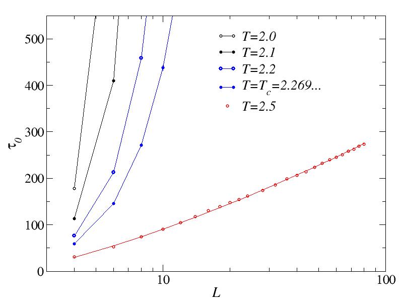
Part 2 (time to reach m=0)

Below Tc, the average time to reach magnetization m=0 diverges exponentially, which we can see by graphing the results on a lin-log scale. Because there is a different behavior exactly at Tc (analyzed below), below Tc but close to Tc we expect the critical behavior to be followed for small systems, before the exponential divergent form sets in. This is seen here from the fact that the pure exponential behavior only sets in above sone cross-over system size which increases as we approach Tc. Here only the T=2.0 and T=2.1 data have been fitted to exponential forms (straight lines on this scale)

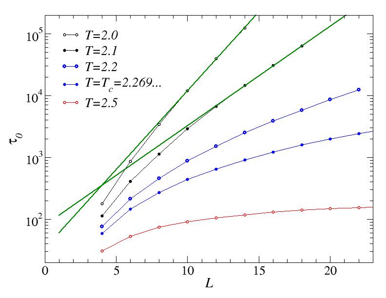
At the critical point we might expect a power-law behavior and therefore plot the data on a log-log scale. At Tc we indeed see a linear dependence. the straight line through the data points correspond to a power-law form t~L^z, with z=2.17, with the exponent recognized as the dynamic exponent for Metropolis dynamics in the 2D Ising model.

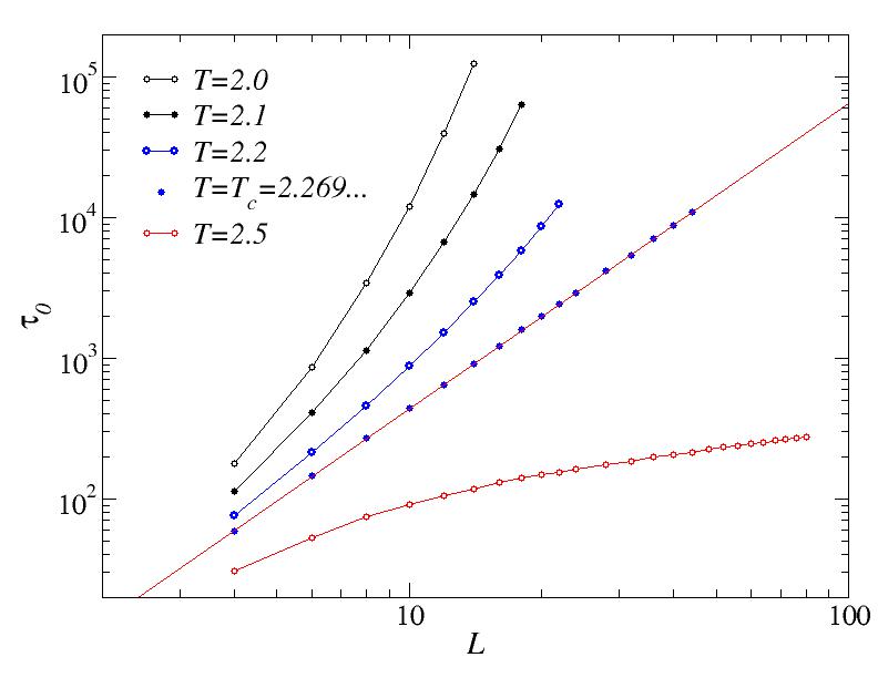
Interestingly, at T = 2.5 > Tc, the time scale still diverges, but only logarithmically. The curve fitted to the T=2.5 data corresponds to the form t=a*ln(L)*b, with the exponent b close to 1.5.