F90 solution program [inertia.f90]
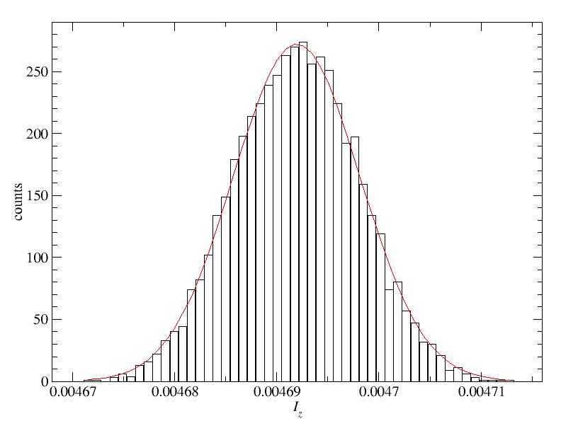
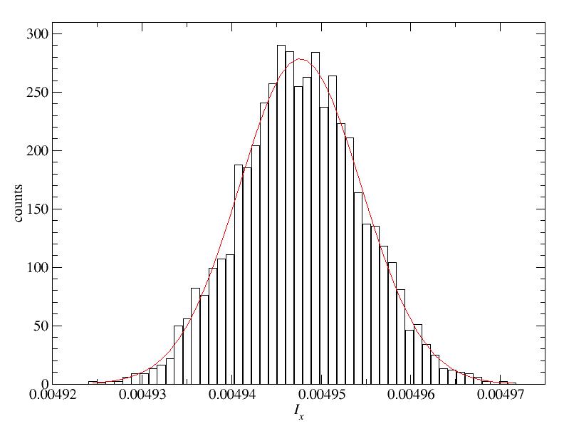
Running the program with 1 million sampling points per bin and nbi bins gave the following results and error bars for Iz and Iynbi = 50: Iz = 0.00469302 +/- 0.00000081, Ix = 0.00494854 +/- 0.00000091 nbi = 500: Iz = 0.00469148 +/- 0.00000027, Ix = 0.00494760 +/- 0.00000031 nbi = 5000: Iz = 0.00469192 +/- 0.00000009, Ix = 0.00494771 +/- 0.00000010Note that when increasing the number of bins by a factor of 10, the error bar is reduced approximately by sqrt(10), as expected statistically. The nbi=5000 run gave bin averages with the following distributions (using 50 histogram bins within the range where data appeared):